Use with PyGMT

Here we demonstrate how to use the figure output from PolarToolkit with normal PyGMT commands. PyGMT offers much more flexibility than PolarToolkit, so if you want to change lots of details of a figure, we recommend using this approach.

%load_ext autoreload
%autoreload 2

from polartoolkit import fetch, maps

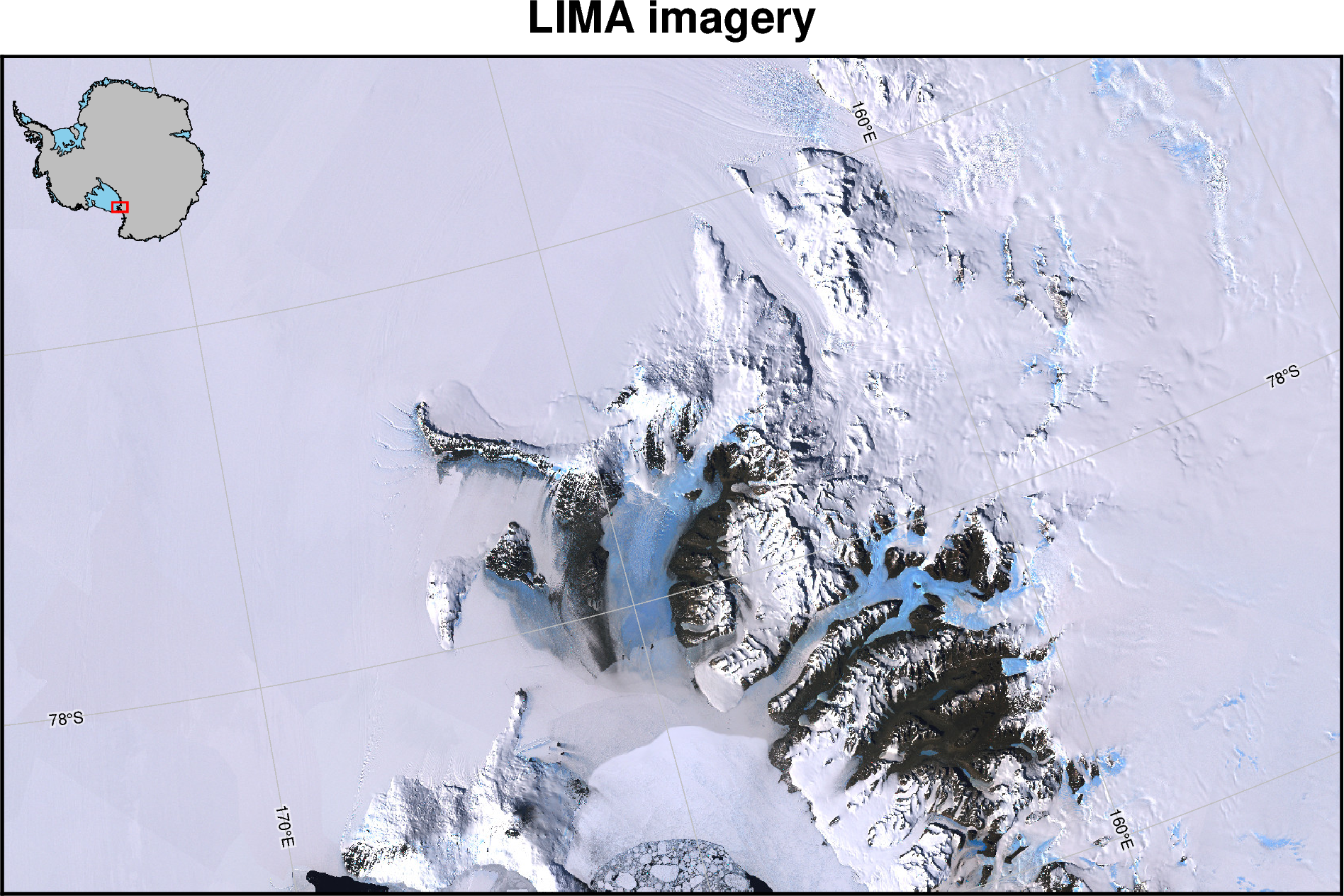
Fetch the datasets, bedmap2 surface topography and LIMA satellite imagery

imagery = fetch.imagery()

surface = fetch.bedmap2(layer="surface")

# define the region of interest
region = (150e3, 550e3, -1350e3, -1100e3)

# plot the imagery and some additional map features
fig = maps.plot_grd(
    imagery,  # GMT automatically recognizes that this is imagery and sets colorscale
    region=region,
    inset=True,
    title="LIMA imagery",
    gridlines=True,
    x_spacing=5,  # plot 10 degree longitude lines
    y_spacing=1,  # plot 2 degree latitude lines
    colorbar=False,
    hemisphere="south",
)

fig.show(dpi=200)

[Session pygmt-session (19)]: Error returned from GMT API: GMT_PTR_IS_NULL (75)
[Session pygmt-session (19)]: Error returned from GMT API: GMT_PTR_IS_NULL (75)
[Session pygmt-session (19)]: Error returned from GMT API: GMT_PTR_IS_NULL (75)
[Session pygmt-session (19)]: Error returned from GMT API: GMT_OBJECT_NOT_FOUND (60)
NULL pointer access
clipping grid to plot region failed!
gmtset [WARNING]: Representation of font type not recognized. Using default.

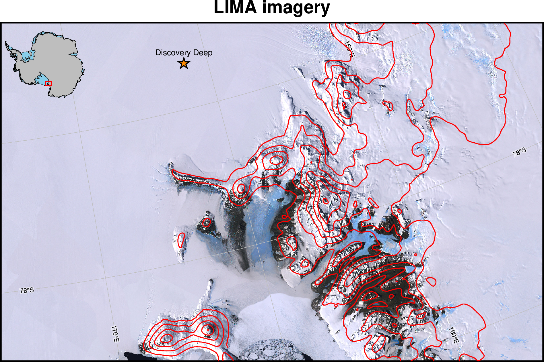
Use additional PyGMT plotting methods on the figure

# add surface elevation contours
fig.grdcontour(grid=surface, levels=500, pen="thick,red")

# add a point and label
fig.plot(x=285000, y=-1130000, style="a0.5c", pen="1p,black", fill="darkorange")
fig.text(x=285000, y=-1130000, text="Discovery Deep", offset="0c/.5c")

# show the figure
fig.show(dpi=200)