Extract and plot data along a profile#
The module polartoolkit.profiles provides convenient tools to extract data along a profile, and automatically create plots of the results. These plots can optionally include a map, a cross section of earth layers, and a profile of other datasets.
There are 3 methods to define the location of the profile: “Points”, “Shapefile”, and “Polyline”
[21]:
%load_ext autoreload
%autoreload 2

import os

from polartoolkit import fetch, profiles, utils
The autoreload extension is already loaded. To reload it, use:
  %reload_ext autoreload
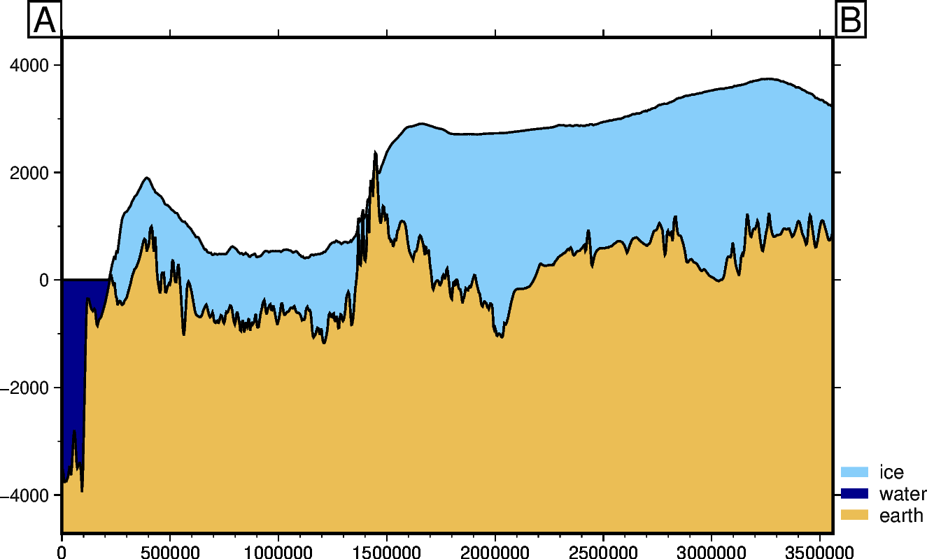
Method 1: “Points”#
define a start and end point for a profile, in EPSG:3031 projection. See the Defining Regions for a map with EPSG gridlines. Sample bedmap2 layers between these points, and plot the cross section. Also set a temporary environment variable to tell PolarToolkit all the code in this notebook is related to the southern hemisphere, instead of the northern.
[2]:
os.environ["POLARTOOLKIT_HEMISPHERE"] = "south"
a = (-1200e3, -1400e3)
b = (1000e3, 1400e3)
[3]:
# this functions returns the figure as well as 2 dataframe with the sampled layers and
# sampled data
fig, df_layers, df_data = profiles.plot_profile(
    method="points",
    start=a,
    stop=b,
)
fig.show(dpi=200)
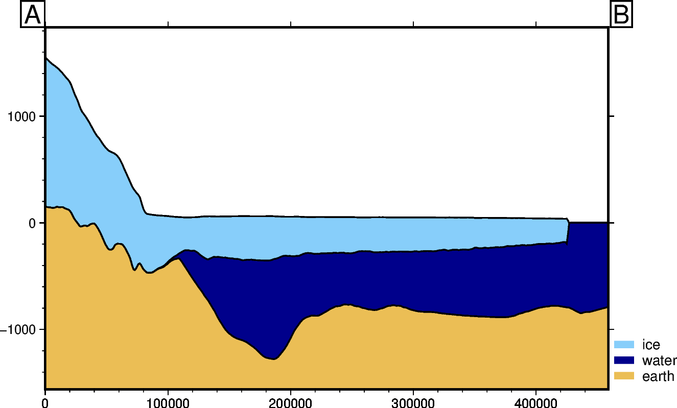
Method 2: “Shapefile”:#
Instead of using a line defined by 2 points, we can sample along the path of a shapefile. Provide a file name, or load a already included shapefile with the function fetch.
Here is a curved path across the Ross Ice Shelf from Mulock Glacier to the ice front through Discovery Deep.
[4]:
fig, _, _ = profiles.plot_profile(
    method="shapefile",
    shapefile=fetch.sample_shp("Disco_deep_transect"),
    fillnans=True,
)
fig.show(dpi=200)
Downloading data from 'doi:10.6084/m9.figshare.26039578.v1/Disco_deep_transect.zip' to file '/home/sungw937/.cache/pooch/polartoolkit/shapefiles/Disco_deep_transect'.
SHA256 hash of downloaded file: 70e86b3bf9775dd824014afb91da470263edf23159a9fe34107897d1bae9623e
Use this value as the 'known_hash' argument of 'pooch.retrieve' to ensure that the file hasn't changed if it is downloaded again in the future.
Unzipping contents of '/home/sungw937/.cache/pooch/polartoolkit/shapefiles/Disco_deep_transect' to '/home/sungw937/.cache/pooch/polartoolkit/shapefiles/Disco_deep_transect.unzip'
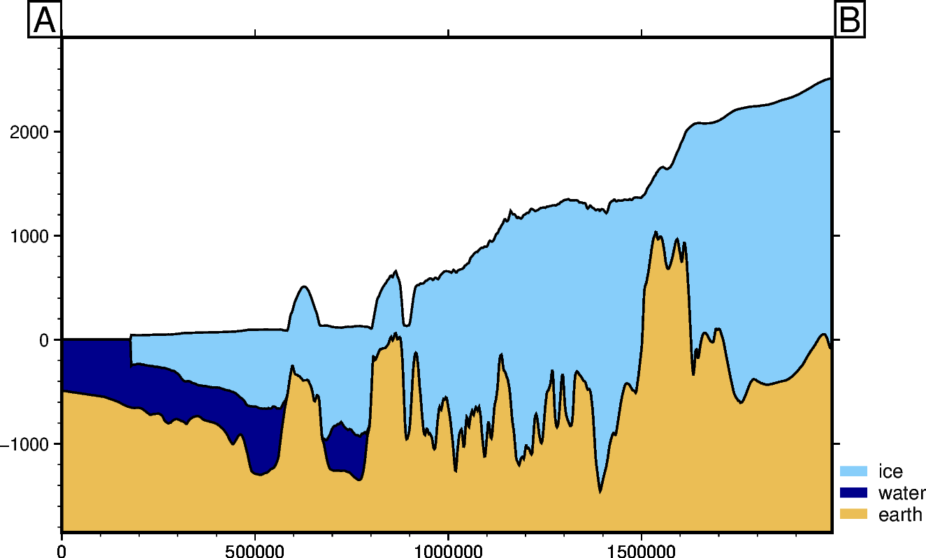
Method 3: “Polyline”:#
Alternatively, load an interactive map, click to create a line, and use that line to create the path.
Note: this requires a few optional dependencies. This can be install with: pip install polartoolkit[interactive] or installed individually with: mamba install geoviews cartopy ipyleaflet ipython
The below cell will display an interactive map of Antarctica. Drag or zoom to your region of interest and use the Draw a polyline button to create the profile you want.
[5]:
lines = profiles.draw_lines()
[7]:
# extract the vertices of the line
df = utils.shapes_to_df(lines)
df
[7]:
| lon | lat | shape_num | easting | northing | |
|---|---|---|---|---|---|
| 0 | -55.848918 | -74.353704 | 0 | -1.415314e+06 | 960081.069463 |
| 1 | -68.853554 | -76.607797 | 0 | -1.363074e+06 | 527236.463707 |
| 2 | -74.711191 | -77.892351 | 0 | -1.273520e+06 | 348128.371368 |
| 3 | -79.070972 | -81.087757 | 0 | -9.526182e+05 | 183945.922942 |
| 4 | -82.619642 | -83.244480 | 0 | -7.287331e+05 | 94391.876850 |
| 5 | -75.781030 | -85.067917 | 0 | -5.197736e+05 | 131706.074346 |
| 6 | -36.022235 | -86.888425 | 0 | -1.988716e+05 | 273500.013170 |
| 7 | -11.423229 | -85.961990 | 0 | -8.692900e+04 | 430219.529909 |
[8]:
# use the line to create a profile, and resample it to get 1000 points
fig, _, _ = profiles.plot_profile(
    method="polyline",
    polyline=df,
    num=1000,
)
fig.show(dpi=200)
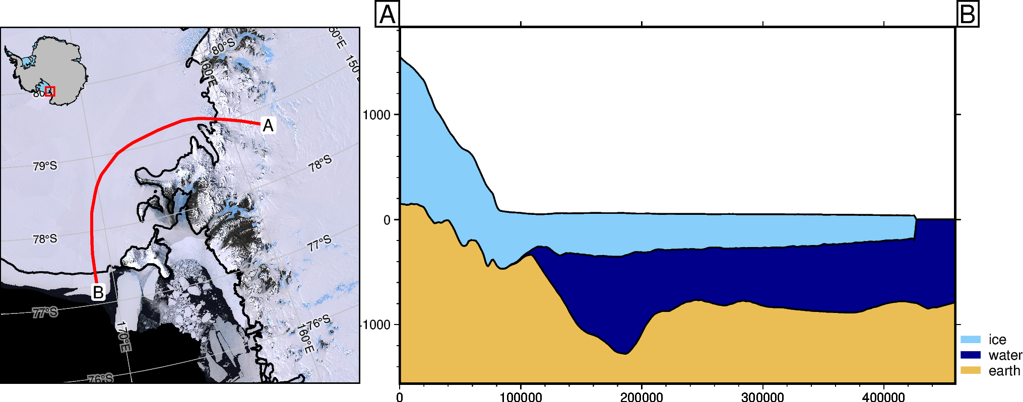
Add a map#
show the profile location by adding a map with a default background of satellite imagery
[9]:
fig, _, _ = profiles.plot_profile(
    method="shapefile",
    shapefile=fetch.sample_shp("Disco_deep_transect"),
    add_map=True,
)
fig.show(dpi=200)
gmtset [WARNING]: Representation of font type not recognized. Using default.
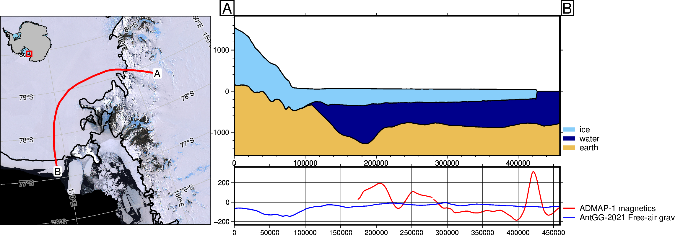
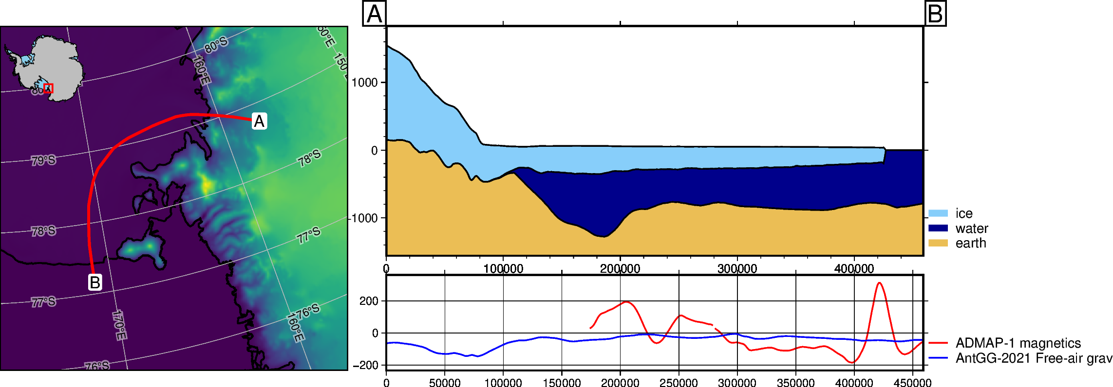
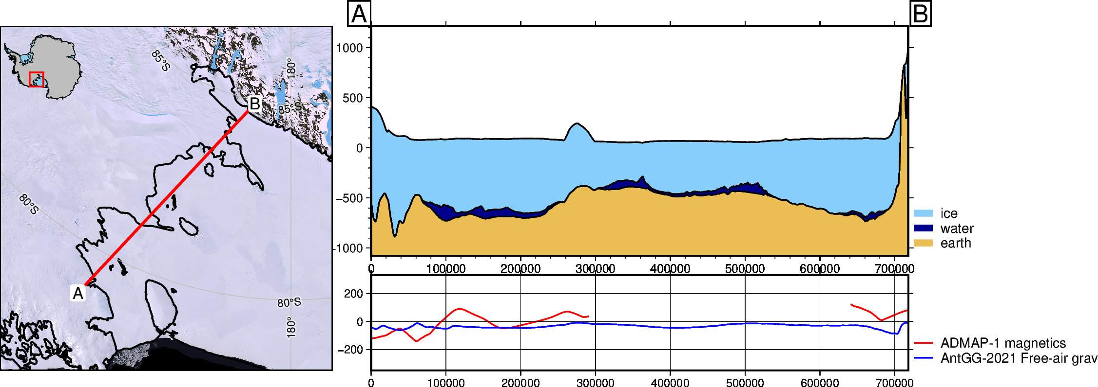
Add a graph of data#
Sample and plot additional datasets along the same profile with data_dict. By default this includes gravity and magnetics.
[10]:
fig, _, _ = profiles.plot_profile(
    method="shapefile",
    shapefile=fetch.sample_shp("Disco_deep_transect"),
    add_map=True,
    data_dict="default",
    legend_loc="JTR+jTR+o.2c/-6c",  # change the default legend location with GMT format
    save=True,  # save the plot to use in README
    path="../cover_fig.png",
)
fig.show(dpi=200)
gmtset [WARNING]: Representation of font type not recognized. Using default.
Change profile length#
clip the profile (either end) based on distance
[11]:
fig, _, _ = profiles.plot_profile(
    method="shapefile",
    shapefile=fetch.sample_shp("Disco_deep_transect"),
    data_dict="default",
    add_map=True,
    min_dist=50e3,
    max_dist=200e3,
    legend_loc="JTR+jTR+o.2c/-6c",  # change the default legend location with GMT format
)
fig.show(dpi=200)
gmtset [WARNING]: Representation of font type not recognized. Using default.
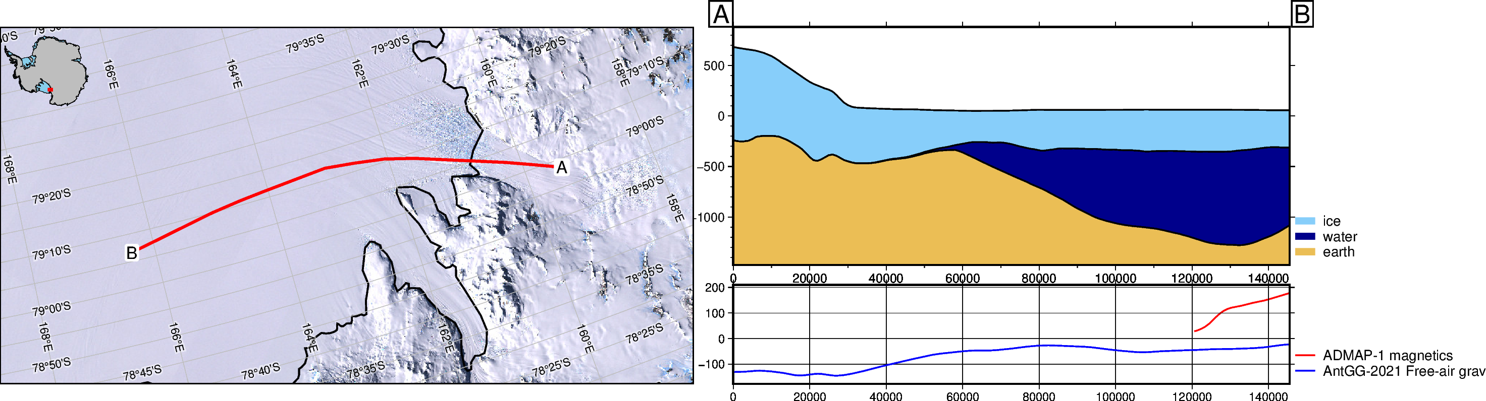
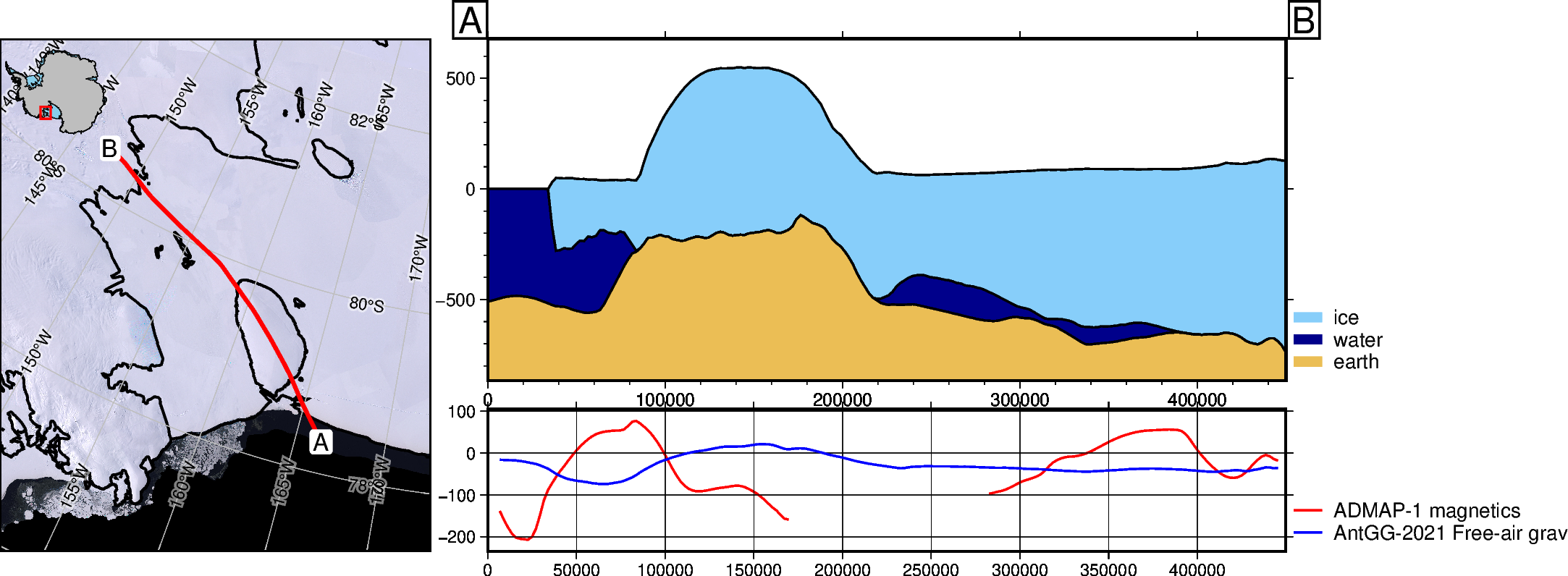
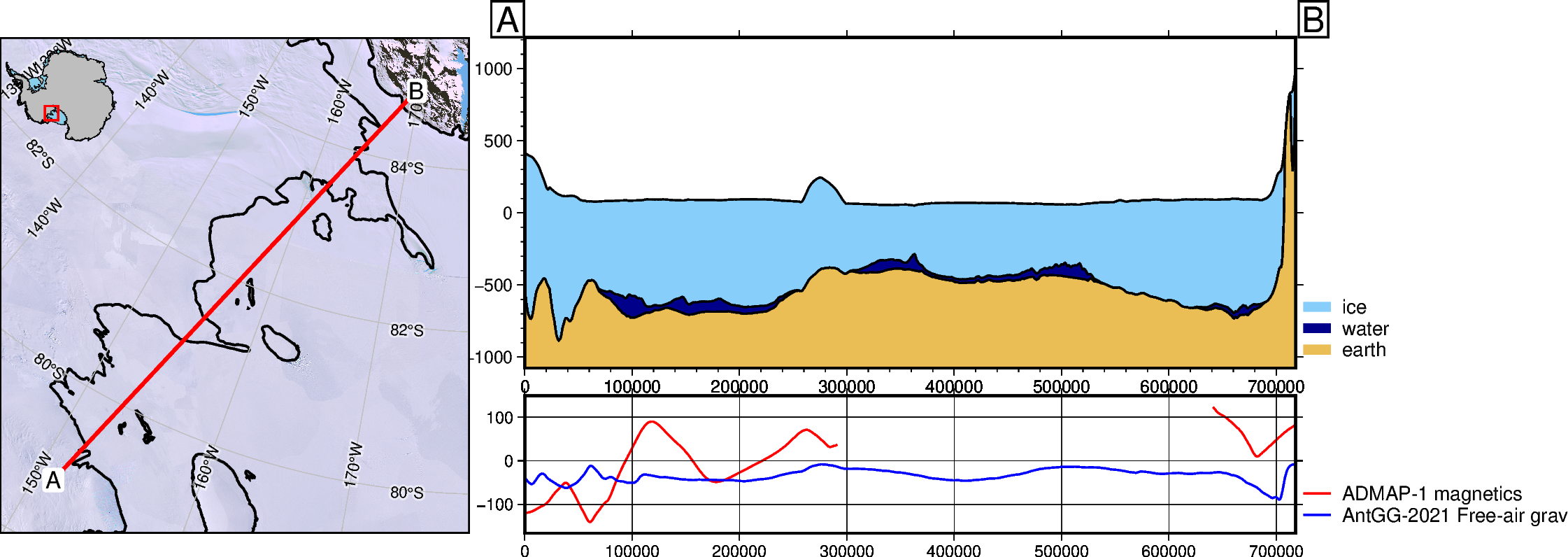
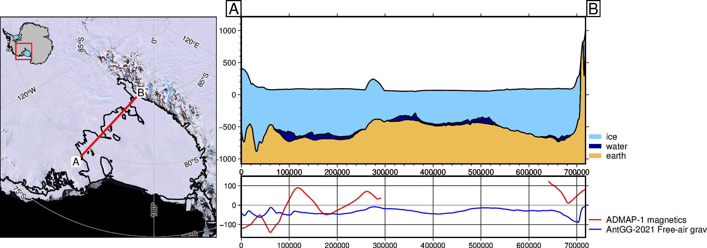
Change sampling resolution#
increase the resolution of the sampling. If using a profile defined by 2 points, use parameter “num”, which defaults to 100 points along the line.
[12]:
fig1, _, _ = profiles.plot_profile(
    method="shapefile",
    shapefile=fetch.sample_shp(
        "Roosevelt_Island",
    ),
    num=30,
    data_dict="default",
    add_map=True,
    legend_loc="JTR+jTR+o.2c/-6c",  # change the default legend location with GMT format
)
fig1.show(dpi=200)

fig2, _, _ = profiles.plot_profile(
    method="shapefile",
    shapefile=fetch.sample_shp(
        "Roosevelt_Island",
    ),
    num=200,
    data_dict="default",
    add_map=True,
    legend_loc="JTR+jTR+o.2c/-6c",  # change the default legend location with GMT format
)
fig2.show(dpi=200)
Downloading data from 'doi:10.6084/m9.figshare.26039578.v1/Roosevelt_Island.zip' to file '/home/sungw937/.cache/pooch/polartoolkit/shapefiles/Roosevelt_Island'.
SHA256 hash of downloaded file: 83434284808d067b8b18b649e41287a63f01eb2ce581b2c34ee44ae3a1a5ca2a
Use this value as the 'known_hash' argument of 'pooch.retrieve' to ensure that the file hasn't changed if it is downloaded again in the future.
Unzipping contents of '/home/sungw937/.cache/pooch/polartoolkit/shapefiles/Roosevelt_Island' to '/home/sungw937/.cache/pooch/polartoolkit/shapefiles/Roosevelt_Island.unzip'
grdtrack [WARNING]: Some input points were outside the grid domain(s).
grdtrack [WARNING]: Some input points were outside the grid domain(s).
gmtset [WARNING]: Representation of font type not recognized. Using default.

grdtrack [WARNING]: Some input points were outside the grid domain(s).
grdtrack [WARNING]: Some input points were outside the grid domain(s).
gmtset [WARNING]: Representation of font type not recognized. Using default.
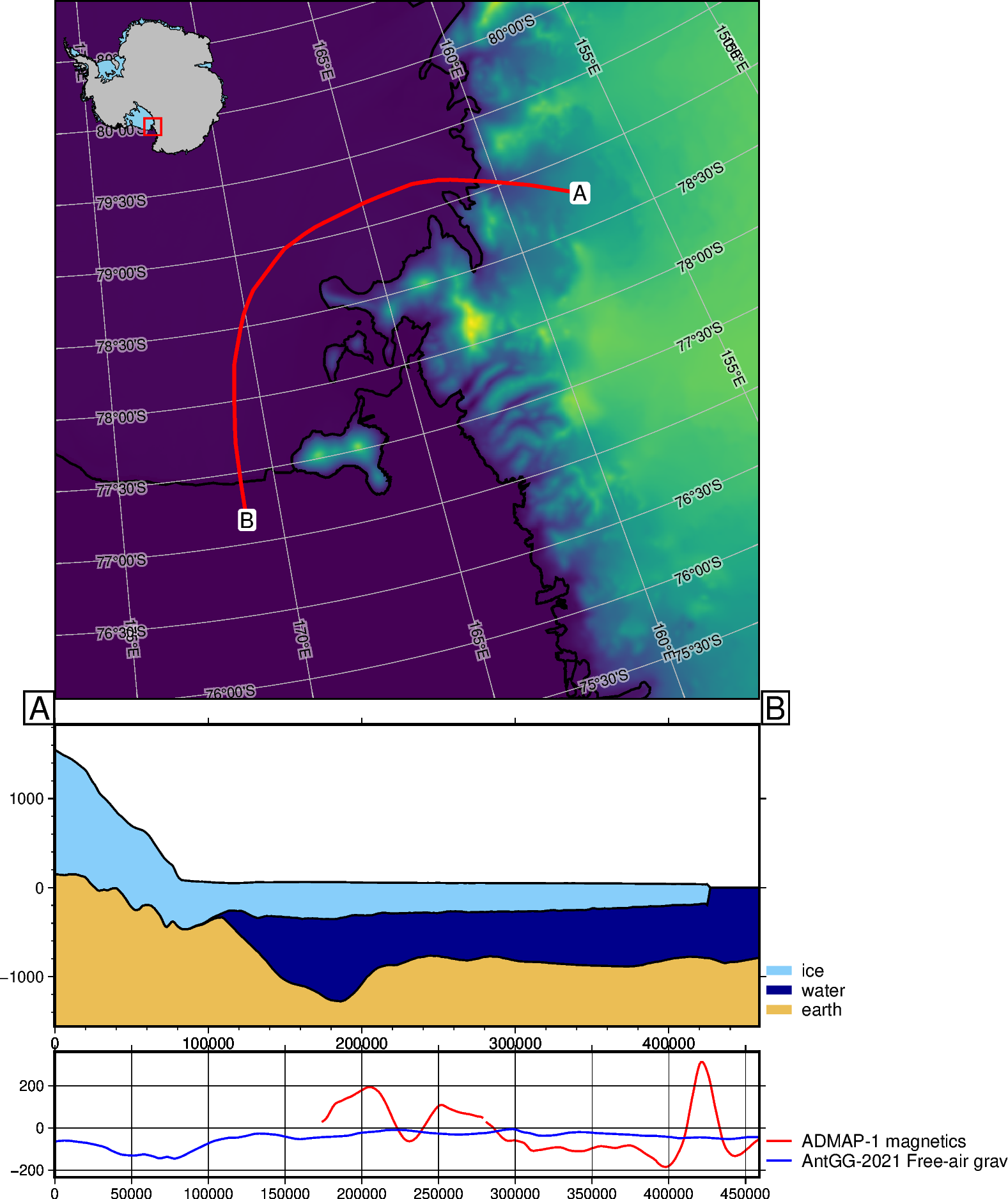
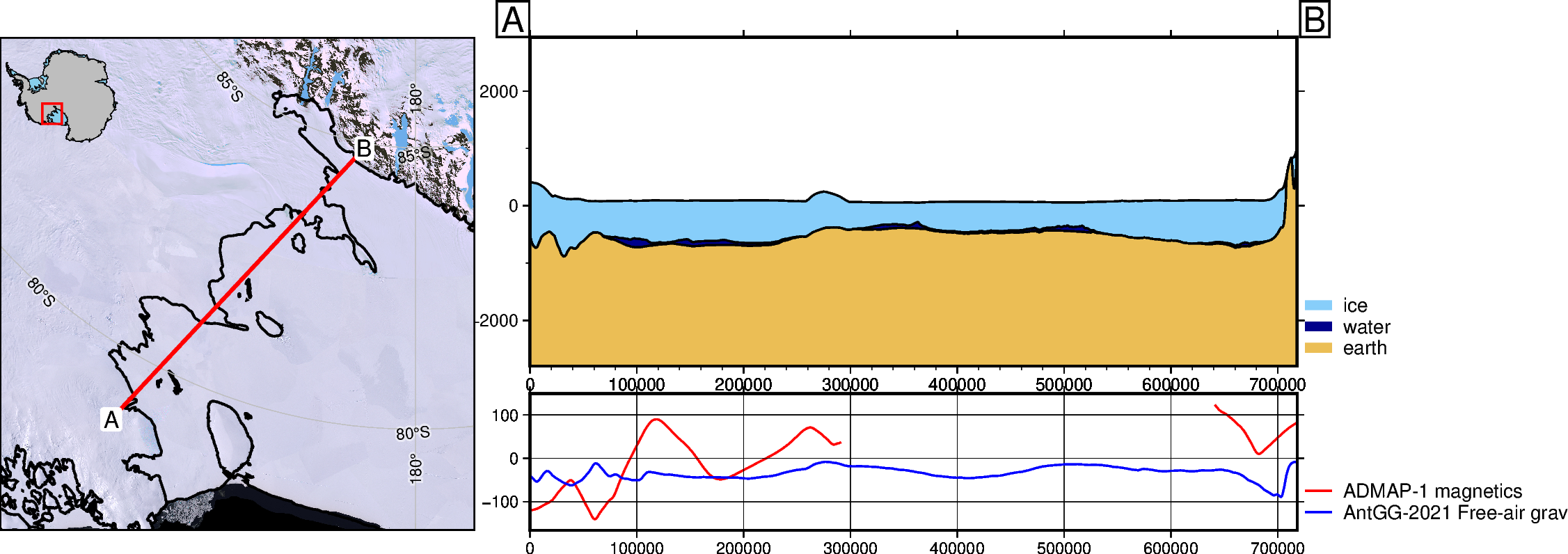
Alter map properies#
Use map_background to change the grid shown on the map. Here, instead of the default imagery, we will show the surface topography from bedmap2.
Also, use subplot_orientation to stack the plots vertically
[13]:
fig, _, _ = profiles.plot_profile(
    method="shapefile",
    shapefile=fetch.sample_shp("Disco_deep_transect"),
    data_dict="default",
    add_map=True,
    map_background=fetch.bedmap2("surface", fill_nans=True),
    subplot_orientation="vertical",
    legend_loc="JTR+jTR+o.2c/-6c",  # change the default legend location with GMT format
)
fig.show(dpi=200)
gmtset [WARNING]: Representation of font type not recognized. Using default.
Use map_cmap to change the maps colorscale
[14]:
fig, _, _ = profiles.plot_profile(
    method="shapefile",
    shapefile=fetch.sample_shp("Disco_deep_transect"),
    data_dict="default",
    add_map=True,
    map_background=fetch.bedmap2("surface", fill_nans=True),
    map_cmap="viridis",
    legend_loc="JTR+jTR+o.2c/-6c",  # change the default legend location with GMT format
)
fig.show(dpi=200)
gmtset [WARNING]: Representation of font type not recognized. Using default.
Use map_buffer to change the level of zoom on the map. This is a percentage of total line distance, which defaults to 0.3 (130%) of profile length. So if the profile is 100km long, the default map will be 130km along the longest axis.
[15]:
# define new profile endpoints
a = (-590e3, -1070e3)
b = (-100e3, -545e3)

fig1, _, _ = profiles.plot_profile(
    method="points",
    start=a,
    stop=b,
    data_dict="default",
    add_map=True,
    map_buffer=0.1,
    legend_loc="JTR+jTR+o.2c/-6c",  # change the default legend location with GMT format
)
fig1.show(dpi=200)

fig2, _, _ = profiles.plot_profile(
    method="points",
    start=a,
    stop=b,
    data_dict="default",
    add_map=True,
    map_buffer=0.8,
    legend_loc="JTR+jTR+o.2c/-6c",  # change the default legend location with GMT format
)
fig2.show(dpi=200)
gmtset [WARNING]: Representation of font type not recognized. Using default.
gmtset [WARNING]: Representation of font type not recognized. Using default.
Alter Cross-section properties#
Use layer_buffer to alter the amount of whitespace above and below the cross-section layers, this defaults to 0.1 (10% of data spread added above/below)
[16]:
fig, _, _ = profiles.plot_profile(
    method="points",
    start=a,
    stop=b,
    data_dict="default",
    add_map=True,
    layer_buffer=1.0,
    legend_loc="JTR+jTR+o.2c/-6c",  # change the default legend location with GMT format
)
fig.show(dpi=200)
gmtset [WARNING]: Representation of font type not recognized. Using default.
Use data_buffer to alter the whitespace above and below data graph, defaults to 0.1 (10% of data spread added above/below)
[17]:
fig, _, _ = profiles.plot_profile(
    method="points",
    start=a,
    stop=b,
    data_dict="default",
    add_map=True,
    data_buffer=0.8,
    legend_loc="JTR+jTR+o.2c/-6c",  # change the default legend location with GMT format
)
fig.show(dpi=200)
gmtset [WARNING]: Representation of font type not recognized. Using default.
Custom layers, datasets, and colors#
The input for both the data and the layers are nested dictionaries, where each dictionary entry contains keys: ‘name’, ‘grid’, and ‘color’.
Use the function, profiles.make_data_dict() to help create these dictionaries. It takes 3 inputs, which are:
a list of names
a list of grids either geotiff/netcdf file names or xarray.DataArrays
a list of colors.
For example, if you have a netcdf file ‘ice_velocity.nc’ which you want to plot as orange, you can make that into a dictionary with: profiles.make_data_dict(['ice velocity'], ['ice_velocity.nc'], ['orange'])
Optionally, you can use Pooch.fetch to help download and store dataset from urls, and easily load them.
See the functions in the module polartoolkit.fetch for examples and feel free to make a PR and add your datasets there.
[22]:
# note, these datafile can be plotted at higher resolution by adding parameter 'spacing'
# to the 'fetch' function:
# fetch.gravity(version="antgg-update", anomaly_type="BA", spacing=1e3) will use a 1km
# version of the Bouguer gravity anomaly.
data_dict = profiles.make_data_dict(
    ["Bouguer gravity", "REMA surface elevation"],
    [
        fetch.gravity(
            version="antgg-2021",
            anomaly_type="BA",
        ).bouguer_anomaly,
        fetch.rema(version="1km"),
    ],
    ["purple", "red"],
    axes=[0, 1],
)

# get default bedmap2 layers
layers_dict = profiles.default_layers(version="bedmap2")

# get grid from basement topography
bed = fetch.bedmap2(layer="bed")
sed_thickness = fetch.sediment_thickness(version="tankersley-2022")
basement = utils.grd_compare(bed, sed_thickness, plot=False)[0]

# add dictionary entry of extra layer 'basement'
layers_dict["basement"] = {}
layers_dict["basement"]["name"] = "basement"
layers_dict["basement"]["grid"] = basement
layers_dict["basement"]["color"] = "chocolate"
[23]:
a = (-590e3, -1070e3)
b = (-150e3, -600e3)

fig, _, _ = profiles.plot_profile(
    "points",
    start=a,
    stop=b,
    add_map=True,
    data_dict=data_dict,
    layers_dict=layers_dict,
    legend_loc="JTR+jTR+o.2c/-6.3c",  # change the default legend location
)
fig.show(dpi=200)
gmtset [WARNING]: Representation of font type not recognized. Using default.
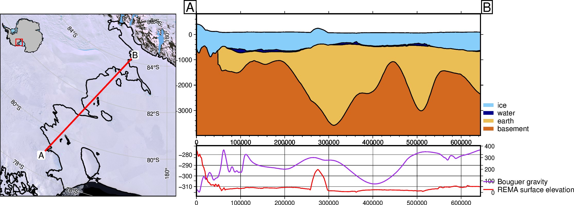
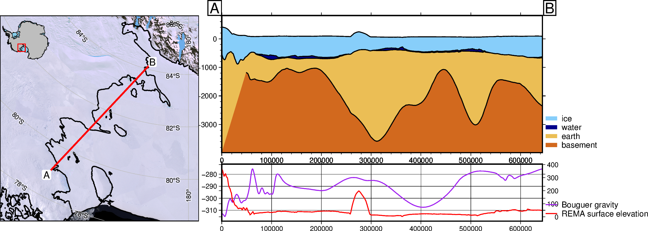
Control wheather to fill gaps in the cross-section layers. Note that the additional layer ‘basement’, doesn’t extend past the groundingline. By default, NaN’s in any layer are set equal to the layer above, causing the vertical line at ~100km.
[24]:
fig, _, _ = profiles.plot_profile(
    "points",
    start=a,
    stop=b,
    add_map=True,
    data_dict=data_dict,
    layers_dict=layers_dict,
    fillnans=False,
    legend_loc="JTR+jTR+o.2c/-6.3c",  # change the default legend location
)
fig.show(dpi=200)
gmtset [WARNING]: Representation of font type not recognized. Using default.
[ ]: