8. Create a cross-section and profile#
PolarToolkit provides some tools for extracting data along a line and plotting it. If the data is topographic, cross-sections of the Earth can be. Other types of data can also be extracted and plotted. Here we demonstrate the basic use of these functions.
[1]:
%load_ext autoreload
%autoreload 2

import os

from polartoolkit import profiles
[2]:
# set default to southern hemisphere for this notebook
os.environ["POLARTOOLKIT_HEMISPHERE"] = "south"
Define the profile as a straight line between two points. Each point is defined by a set of coordinates in meters east and north from the pole in the EPSG 3031 projection.
[3]:
# meters east and north of the south pole in EPSG 3031
a = (1925000, 830000)
b = (2200000, 600000)
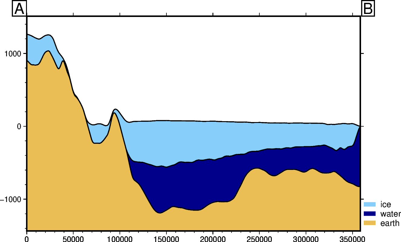
[4]:
fig, df_layers, _ = profiles.plot_profile(
    method="points",
    start=a,
    stop=b,
    default_layers_spacing=5e3,
)
fig.show(dpi=200)
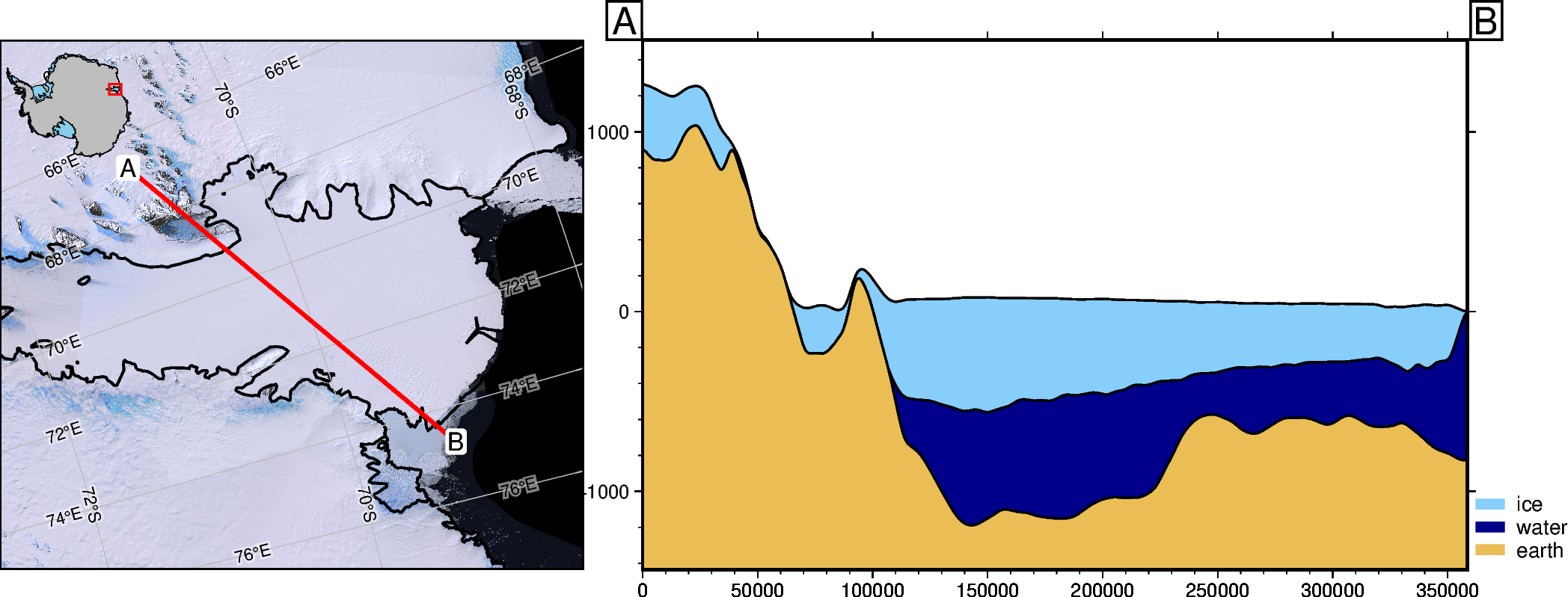
To see where in Antarctica this is, we can add a map showing the profile location.
[5]:
fig, _, _ = profiles.plot_profile(
    method="points",
    start=a,
    stop=b,
    add_map=True,
    default_layers_spacing=5e3,
)
fig.show(dpi=200)
gmtset [WARNING]: Representation of font type not recognized. Using default.
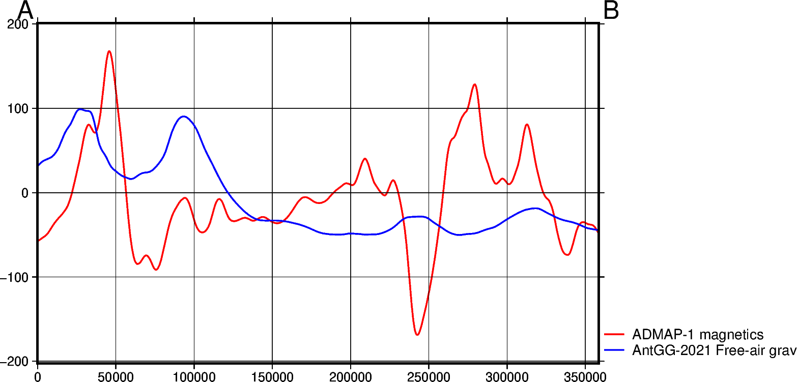
We can also extract non-topographic data along the same line and plot it with the plot_data function. Here we use some default data from PolarToolkit which consists of gravity and magnetic anomaly data.
[6]:
fig, _ = profiles.plot_data(
    method="points",
    start=a,
    stop=b,
    data_dict="default",
)
fig.show(dpi=200)
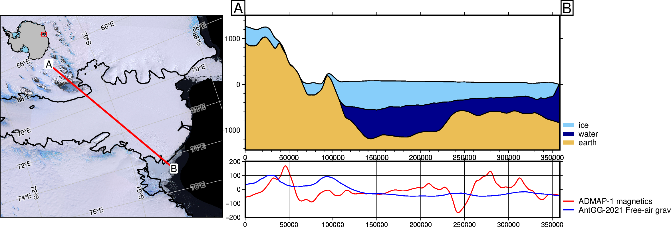
This can also be added within the plot_profile function.
[7]:
fig, _, _ = profiles.plot_profile(
    method="points",
    start=a,
    stop=b,
    add_map=True,
    data_dict="default",
    default_layers_spacing=5e3,
)
fig.show(dpi=200)
gmtset [WARNING]: Representation of font type not recognized. Using default.
For more specifics on use profiles in PolarToolkit see this how-to guide.